It's Raining Photons

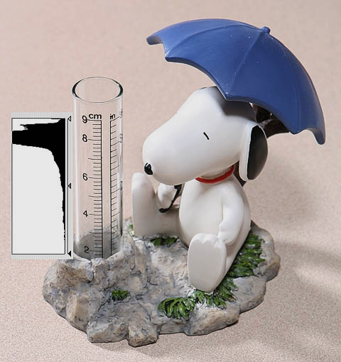
The sensor of a digital camera is like an array of buckets, but instead of holding water they capture photons and convert them to voltage levels. Like a bucket each sensor site has a finite capacity and those in highlight areas fill to capacity before those in the shadows. Camera metering tries to predict in advance of the actual exposure, with varying degrees of success, when the sensor in the brightest highlights will get maxed out and require closing the shutter to end the exposure.

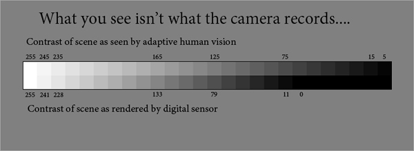
The greatest physical limitation in the photographic process is that color film and digital sensors can't record the same range of brightness that our eyes can detect. In a digital camera the shutter closes to end the exposure before the sensor cells in the darkest areas have absorbed enough photons to record an image. Our eyes can detect difference in tone over about a 10-11 f/stop range of brightness but a digital camera can only record about a 7-stop range with discernible detail on screen or print:

The biggest difference between how our eye see and a camera records the scene is how the pupil of the eye adapts to the light level as it moves around the scene. The pupil will dilate in when focusing on darker areas and constrict when looking at brighter ones. The brain stitches all the snippets into a panoramic mosaic we perceive as well exposed. The camera lens records the entire scene at one aperture per shot. If exposure is optimized for the highlights then shadow detail is lost, compared to our baseline for "normal"; what is perceived by eye.

In the shot below the exposure was optimized for the highlight detail in the sunlit parts of the white towel, and due to the range limit of the camera the middle tones look darker than expected and there is a loss of shadow detail:

The Histogram

The width of the histogram chart always represents the range of the sensor from 0 (black) to 255 (specular highlight white). The contents of the chart is actually a bar graph consisting of 256 bars representing 256 discrete tones in the final reproduction: a zone system consisting of 255 zones. The vertical amplitude of the bars indicate, how many pixels in the display JPG were exposed to create that tone in the final reproduction. Combined, the bars on the graph show visually how the range of the scene fits the range of the sensor.

The measurement is done after the exposure as the image is processed and a JPG file for the display is created. It is important to realize the histogram is based on the display JPG not the RAW capture which has a longer overall range.

The horizontal axis of the histogram represents 256 levels of brightness, from 0 on the extreme left to 255 on the extreme right. The vertical axis of the histogram represents how many pixels in the image have that value.

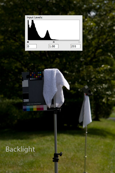
Optimal exposure, in the technical sense, occurs when the brightest and darkest areas with detail barely touch the two sides of the histogram, as in this studio lighting test shot:

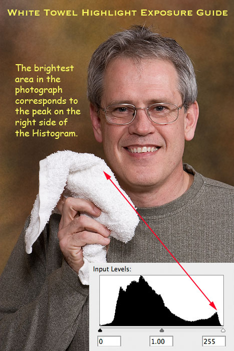
The photographer's eyes and brain play an important part in interpreting the histogram. Understanding what the histogram is revealing about the scene requires visually identifying the lightest and darkest objects in the scene then correlating them to the position of peaks on the right and left sides of the horizontal histogram scale.

Setting Highlight Exposure Using the Right Side of the Histogram

Every scene, even predominantly dark ones, have important highlight detail. Many of the subtle clues the brain uses to discern 3D shape from contrast patterns in a photo come from the details recorded around the bright specular highlights. So the challenge for the photographer is to keep the highlights exposed so clipping, if it occurs at all, is only happening in mirror-like specular reflection.

Exposure can be controlled various ways. The three basic camera controls are ISO speed, shutter and aperture. When artificial lighting is used the power level of the lighting can also be used to modulate exposure. In the automatic metering modes on the Canon cameras I use (P, Av, Tv) Exposure Compensation (EC) is used to override the default camera metering "guess" of exposure. When automatic flash metering is used (ETTL mode on Canon flash) the flash metered power level can be over-ridden with Flash Exposure Compensation (FEC).

Regardless of the method use the goal should be to shift the histogram bars to the right until white textured highlights
are just below clipping to reproduce them normally with detail. The problem with using a Histogram for adjusting highlight exposure is that many scenes do not have any white highlights areas which are large enough to register on the vertical scale of the graph. That's why whenever possible I include a white terry towel in my test shots as a proxy for the smaller areas which do not display well on the histogram:

The reason I use a towel rather than a smooth object like a card is because it is easier to detect visually when over-exposure starts to erode highlight detail. Note the position of the peak the range of highlight tones in the towel creates on the right side. By comparison of the camera histogram with how the files with the towel guide look in the RAW file I am able to gauge from the appearance on the camera playback what is happening in the highlights of the RAW file. I don't try to keep exposure on the "bleeding edge" of clipping during capture, preferring instead to have some leeway for highlight adjustment in the editing stages.

Notice above how matching the range of the scene to the sensor results in a very natural appearance? That's the magic of the photographic process. When exposure is controlled with camera settings and lighting so both ends are reproduced correctly, everything in-between winds up looking how it is perceived by eye normally. Its only when the range does not fit the sensor and highlight or shadow detail is lost that photographs look fake.

The Over-Exposure Warning (OEW)

When I started exposing for highlight detail using the white towel I noticed a correlation between when the black-out clipping warning in the highlights appeared playback and loss of detail in towel the RAW file. Because the shows exactly where clipping is occurring it is a better tool for judging highlight exposure than the histogram. The OEW also works better on white backgrounds. So I now primarily rely on the OEW to set optimal highlight exposure then look at the left side of the Histogram.

Reproduction of Midtones and Shadows

As seen in this backlit outdoor scene, when the range of the scene exceeds the range of the sensor and exposure is set to retain the highlight detail the middle tones and shadows are rendered darker than normally perceived by eye.

That has been a fact of photographic life since the introduction of color film in the 1940s. Photographers learned to cope several ways. If only ambient light is available a portrait subject would be placed back to the sun and exposure set not for the highlights, but to reproduce the shaded face normally. The downside of that "perceptual" approach to exposure is the loss of highlight detail in the hair, bare arms, light clothing and the sky. Another way to cope with outdoor lighting which exceeds the sensor range is to shoot into the shadow side of the ambient then add flash to lift up the shaded side, a process commonly referred to as "fill flash". Here is the scene above with flash added to make the front of the foreground look more "normal" (i.e. what is expected) relative to the context of the background.

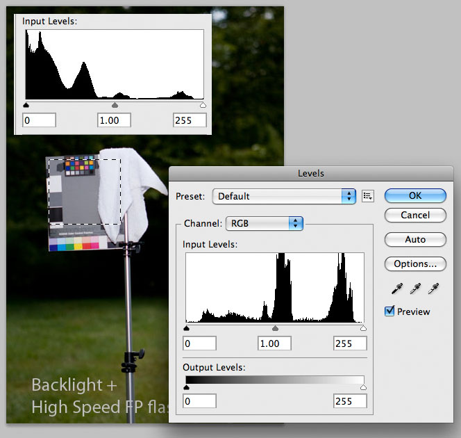
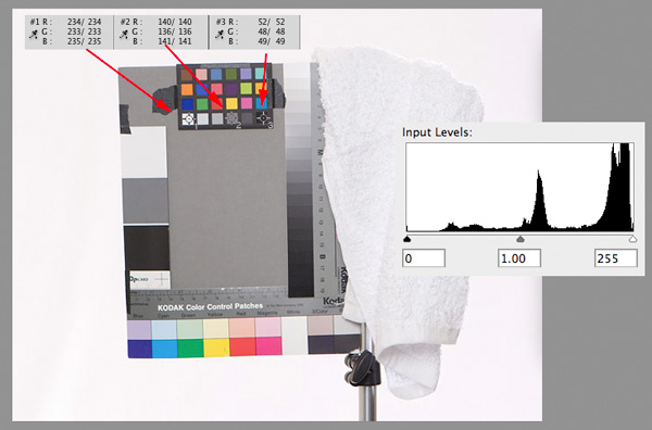
As can be seen from the histograms the overall scene histogram (top) still shows the left side piled up and running off the scale, indicating a loss of shadow detail. But the histogram of just the target in the foreground reveals it is optimally exposed with both ends of the graph just touching the right and left edges. Here is an outdoor portrait make with the same exposure strategy of shooting into the shadows and exposing ambient below clipping then adding flash to raise the level of the foreground to what is perceived as "normal":

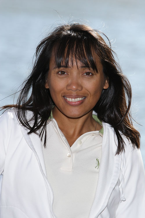
What you should notice and grasp about "fill flash" is the fact that the flash is actually working in the role of key light creating the highlight pattern on the face. The shadow areas not hit by the flash remain filled by the ambient light bounced off the sky the subject is facing. I explain this in depth in other tutorials.

Calibrating Your Brain to Understand the Histogram

As mentioned the Histogram, like any form of exposure measurement, must be interpreted by the photographer to be of any value in controlling exposure creatively. Each spot on the horizontal scale represents a discrete tone of gray between the extremes. Below I show a simple way to create a visual "roadmap" of your camera sensor range as it relates to f/stops. To perform this exercise its best to use:

• Uniform lighting conditions such as outdoor light on a clear sunny day
• A commercial gray card known to be neutral such as the Kodak R-29
• A fast wide-aperture lens
• A tripod

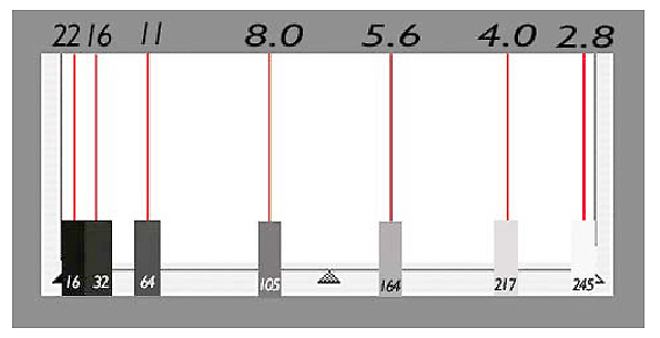
The net result of the exercise will be a facsimile of the histogram showing how the changes in exposure shift the tonal value of the gray card:

Here is the procedure for the exercise

1. Start by arranging the camera so the entire viewfinder is filled with the gray card in uniform light and set custom white balance off the card. Starting by setting custom WB ensures that all three RGB channels will be in sync and the card will be reproduced as neutral gray.

2. Use a lens with wide range of apertures. Put the camera at ISO 100 in M mode in and open your lens to its widest full f/stop (e.g., f/1.4, f/2.0, f/2.8) then find the shutter speed that will make the card image blink indicating over-exposure. We want to start the test by intentionally over-exposing the gray card to just below the point of clipping so increase shutter speed by 1/3 stop (one click of the camera dial) until the blinking in the OEW disappears.

3. Shoot a bracketed series of exposure of the full card, closing the lens aperture by one full 1-f/stop with each frame until you run out of stops on the lens. As you shoot you will notice that the narrow spike the card forms on the histogram marches from right-to-left across the graph. If using a fast lens stopping down to the smallest aperture should be sufficient to move the spike all the way to the left edge. If not, when you run out of apertures start changing shutter speed, doubling it for each successive frame.

4. After shooting the series put a piece of tape on the LCD and mark spots where the spikes occur with a marking pen as you scroll through the images.

I created the illustration above using a screen shot of an empty Levels histogram in Photoshop, adding the red lines to correspond to where the histogram spike was located for each exposure. The gray patches were copied and pasted from each exposure and the small numbers are their RGB values read with the eyedropper tool.

That test performed with my Canon 20D and 24-70mm f/2.8 L lens revealed that there was about a 7-stop range between textured highlight values of 245 and the darkest shadows values of around 30 I can typically see on screen or print. So I know if I expose for the highlight detail and the shadows are causing the histogram to pile-up on the left the scene is contains more than 7 f/stops of brightness difference.

Sensor range varies from camera to camera and due to flare and other factors one lens may produce different results than another. Camera ISO also affects sensor range. It's a very simple test to perform and it only takes a few minutes. Try it and learn more about your camera's range and what its histogram is telling you.